Understanding Underfitting and Overfitting in Machine Learning

Posted by tintin_2003 on 2025-10-08 21:16:47 |

Share: Facebook | Twitter | Whatsapp | Linkedin Visits: 30

Understanding Underfitting and Overfitting in Machine Learning

1. Introduction

Imagine you're preparing for an exam. If you barely glance at the textbook, you'll fail because you didn't learn enough. But if you memorize every single word, punctuation mark, and page number without understanding the concepts, you'll struggle with questions that are worded differently. Machine learning models face this exact dilemma - finding the sweet spot between learning too little (underfitting) and memorizing too much (overfitting).

2. Definition

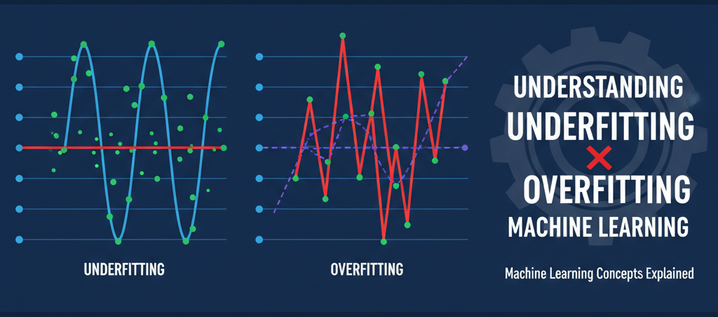
Underfitting occurs when a model is too simple to capture the underlying patterns in the data. It performs poorly on both training data and new, unseen data because it hasn't learned enough from the examples.

Overfitting occurs when a model is too complex and learns not just the patterns but also the noise and random fluctuations in the training data. It performs excellently on training data but fails on new, unseen data because it memorized specific examples rather than learning general patterns.

The Goal: Find the optimal complexity where the model generalizes well to new data while capturing the true underlying patterns.

3. Code

import numpy as np
import matplotlib.pyplot as plt
from sklearn.preprocessing import PolynomialFeatures
from sklearn.linear_model import LinearRegression
from sklearn.metrics import mean_squared_error

# Generate sample data with some noise
np.random.seed(42)
X = np.sort(np.random.rand(30, 1) * 10, axis=0)
y = 2 * X + 3 + np.random.randn(30, 1) * 2  # True relationship: y = 2x + 3 + noise

# Split into train and test
X_train, y_train = X[:20], y[:20]
X_test, y_test = X[20:], y[20:]

# Create models with different complexities
models = {
    'Underfitting (degree=1)': 1,
    'Good Fit (degree=1 with correct approach)': 1,
    'Overfitting (degree=15)': 15
}

# For plotting
X_plot = np.linspace(0, 10, 100).reshape(-1, 1)

plt.figure(figsize=(15, 5))

for idx, (name, degree) in enumerate(models.items(), 1):
    # Create polynomial features
    poly = PolynomialFeatures(degree=degree)
    X_train_poly = poly.fit_transform(X_train)
    X_test_poly = poly.transform(X_test)
    X_plot_poly = poly.transform(X_plot)
    
    # Train model
    model = LinearRegression()
    model.fit(X_train_poly, y_train)
    
    # Predictions
    y_train_pred = model.predict(X_train_poly)
    y_test_pred = model.predict(X_test_poly)
    y_plot_pred = model.predict(X_plot_poly)
    
    # Calculate errors
    train_mse = mean_squared_error(y_train, y_train_pred)
    test_mse = mean_squared_error(y_test, y_test_pred)
    
    # Plot
    plt.subplot(1, 3, idx)
    plt.scatter(X_train, y_train, color='blue', label='Training data', alpha=0.6)
    plt.scatter(X_test, y_test, color='red', label='Test data', alpha=0.6)
    plt.plot(X_plot, y_plot_pred, color='green', linewidth=2, label='Model prediction')
    plt.xlabel('X')
    plt.ylabel('y')
    plt.title(f'{name}\nTrain MSE: {train_mse:.2f}, Test MSE: {test_mse:.2f}')
    plt.legend()
    plt.ylim(-5, 30)

plt.tight_layout()
plt.savefig('underfitting_overfitting.png', dpi=150, bbox_inches='tight')
plt.show()

# Print detailed results
print("=" * 60)
print("MODEL PERFORMANCE COMPARISON")
print("=" * 60)

for name, degree in models.items():
    poly = PolynomialFeatures(degree=degree)
    X_train_poly = poly.fit_transform(X_train)
    X_test_poly = poly.transform(X_test)
    
    model = LinearRegression()
    model.fit(X_train_poly, y_train)
    
    train_mse = mean_squared_error(y_train, model.predict(X_train_poly))
    test_mse = mean_squared_error(y_test, model.predict(X_test_poly))
    
    print(f"\n{name}:")
    print(f"  Training Error: {train_mse:.4f}")
    print(f"  Test Error: {test_mse:.4f}")
    print(f"  Gap (Overfitting indicator): {abs(test_mse - train_mse):.4f}")

4. Real Life Example

The Coffee Shop Story

Imagine you own a coffee shop and want to predict daily sales based on temperature:

Underfitting Example: You create an overly simple rule: "I'll always prepare supplies for 100 cups regardless of temperature." This ignores the clear pattern that people buy more cold drinks when it's hot and more hot drinks when it's cold. Your prediction is consistently wrong, and you either waste supplies or run out of stock. You haven't captured the relationship between temperature and sales at all.

Overfitting Example: You keep extremely detailed records: "On March 15th at 72°F when Mrs. Johnson wore a blue dress, I sold exactly 127 cups." Your prediction system memorizes every tiny detail including irrelevant factors (like what customers wore, if a bird landed on the windowsill, etc.). When a new day comes with similar temperature but different random circumstances, your predictions are wildly inaccurate because you've memorized noise instead of learning the real pattern.

Good Fit Example: You identify the meaningful pattern: "When temperature is 40°F-60°F, I sell around 120 cups (mostly hot drinks). When it's 75°F-90°F, I sell around 150 cups (mostly cold drinks)." This captures the genuine relationship without memorizing irrelevant details, so it works well for new days you haven't seen before.

5. Pseudocode

ALGORITHM: Train Model with Proper Fit

INPUT: 
    training_data (features, labels)
    validation_data (features, labels)
    model_complexity_range

OUTPUT:
    best_model

PROCEDURE:
    1. SPLIT training_data into:
        - actual_training_set (80%)
        - validation_set (20%)
    
    2. FOR each complexity_level IN model_complexity_range:
        
        3. INITIALIZE model with complexity_level
        
        4. TRAIN model on actual_training_set
        
        5. CALCULATE training_error on actual_training_set
        6. CALCULATE validation_error on validation_set
        
        7. IF training_error is HIGH AND validation_error is HIGH:
            → Model is UNDERFITTING
            → Increase complexity
        
        8. ELSE IF training_error is LOW AND validation_error is HIGH:
            → Model is OVERFITTING
            → Decrease complexity or add regularization
        
        9. ELSE IF training_error is LOW AND validation_error is LOW:
            → Model has GOOD FIT
            → Save this model as candidate
        
        10. STORE (complexity_level, training_error, validation_error)
    
    11. SELECT model with lowest validation_error
    
    12. EVALUATE best_model on test_data (completely unseen)
    
    13. RETURN best_model

REGULARIZATION_TECHNIQUE (to prevent overfitting):
    - Add penalty term to loss function
    - Use dropout (randomly disable neurons)
    - Implement early stopping
    - Reduce model complexity
    - Increase training data

6. Mathematics

Loss Function and Model Complexity

The total error of a model can be decomposed as:

Total Error = Bias² + Variance + Irreducible Error

Where:

• Bias: Error from oversimplifying the model (underfitting)
• Variance: Error from being too sensitive to training data (overfitting)
• Irreducible Error: Noise inherent in the data

Mathematical Formulation

Given training data: D = {(x₁, y₁), (x₂, y₂), ..., (xₙ, yₙ)}

We want to find function f(x) that minimizes prediction error.

1. Underfitting (High Bias, Low Variance)

Model is too simple: f(x) = β₀ (just predicting the mean)

Loss function:

L = (1/n) Σᵢ (yᵢ - β₀)²

Training error: High
Test error: High
Problem: Model cannot capture true relationship

2. Good Fit (Balanced Bias-Variance)

Appropriate complexity: f(x) = β₀ + β₁x (for linear relationship)

Loss function:

L = (1/n) Σᵢ (yᵢ - (β₀ + β₁xᵢ))²

Training error: Moderate
Test error: Moderate (≈ training error)
Success: Model captures true underlying pattern

3. Overfitting (Low Bias, High Variance)

Model is too complex: f(x) = β₀ + β₁x + β₂x² + ... + β₁₅x¹⁵ (high-degree polynomial)

Loss function:

L = (1/n) Σᵢ (yᵢ - Σⱼ₌₀¹⁵ βⱼxᵢʲ)²

Training error: Very low
Test error: Very high
Problem: Model memorizes training data including noise

Regularization (Mathematical Solution to Overfitting)

Ridge Regression (L2 Regularization):

L = (1/n) Σᵢ (yᵢ - f(xᵢ))² + λ Σⱼ βⱼ²

LASSO Regression (L1 Regularization):

L = (1/n) Σᵢ (yᵢ - f(xᵢ))² + λ Σⱼ |βⱼ|

Where λ (lambda) is the regularization parameter:

• λ = 0: No regularization (risk of overfitting)
• λ → ∞: Maximum regularization (risk of underfitting)

Expected Test Error Decomposition

For a model f̂(x) trained on dataset D:

E[(y - f̂(x))²] = Bias[f̂(x)]² + Var[f̂(x)] + σ²

Where:

• Bias[f̂(x)] = E[f̂(x)] - f(x): Average deviation from true function
• Var[f̂(x)] = E[(f̂(x) - E[f̂(x)])²]: Sensitivity to training data variations
• σ²: Irreducible noise in data

Underfitting: High Bias, Low Variance
Overfitting: Low Bias, High Variance
Optimal Model: Minimizes Bias² + Variance

This mathematical framework shows that machine learning is fundamentally about finding the sweet spot in the bias-variance tradeoff to achieve the best generalization to unseen data.