Gradient descent — mathematical explanation & full derivation
Machine learning Mathematics in Machine LearningPosted by admin on 2025-09-19 21:24:48 | Last Updated by tintin_2003 on 2026-07-23 01:53:04
Share: Facebook | Twitter | Whatsapp | Linkedin Visits: 355
Gradient Descent: Mathematical Proof and Code Implementation
Mathematical Foundation
1. Basic Setup and Definitions
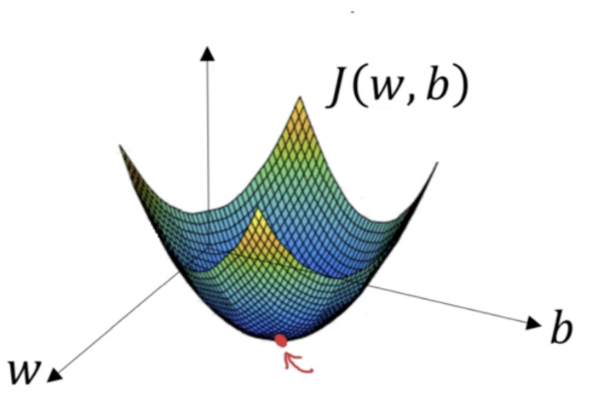
Let f(x) be a differentiable function we want to minimize, where x ∈ R^n.

Goal: Find x* such that f(x*) = min f(x)

Key Insight: The gradient ∇f(x) points in the direction of steepest ascent.
Therefore, -∇f(x) points in the direction of steepest descent.
2. The Gradient Descent Algorithm
Update Rule: x_{k+1} = x_k - α∇f(x_k)

Where:
- x_k is the current point at iteration k
- α > 0 is the learning rate (step size)
- ∇f(x_k) is the gradient at x_k
3. Mathematical Proof of Convergence
Assumptions:
1. f is continuously differentiable
2. f has Lipschitz continuous gradient with constant L > 0:
   ||∇f(x) - ∇f(y)|| ≤ L||x - y|| for all x, y
3. f is bounded below: f(x) ≥ f* for all x
4. Learning rate satisfies: 0 < α < 2/L
Proof:
Step 1: Show that the function value decreases at each iteration
Using Taylor expansion around x_k:

f(x_{k+1}) = f(x_k - α∇f(x_k))
           ≤ f(x_k) + ∇f(x_k)^T(-α∇f(x_k)) + (L/2)||(-α∇f(x_k))||²
           = f(x_k) - α||∇f(x_k)||² + (Lα²/2)||∇f(x_k)||²
           = f(x_k) - α(1 - Lα/2)||∇f(x_k)||²

Since 0 < α < 2/L, we have (1 - Lα/2) > 0, so:

f(x_{k+1}) ≤ f(x_k) - α(1 - Lα/2)||∇f(x_k)||²
Step 2: Show convergence of gradient to zero
Rearranging the inequality:
α(1 - Lα/2)||∇f(x_k)||² ≤ f(x_k) - f(x_{k+1})

Summing from k = 0 to K-1:
α(1 - Lα/2) Σ(k=0 to K-1) ||∇f(x_k)||² ≤ f(x_0) - f(x_K)

Since f is bounded below:
α(1 - Lα/2) Σ(k=0 to K-1) ||∇f(x_k)||² ≤ f(x_0) - f* < ∞

This implies: Σ ||∇f(x_k)||² < ∞
Therefore: ||∇f(x_k)|| → 0 as k → ∞
Step 3: Convergence rates
For convex functions:
f(x_k) - f* ≤ ||x_0 - x*||² / (2αk)
This gives O(1/k) convergence rate.

For strongly convex functions with parameter μ > 0:
||x_k - x*||² ≤ ((L-μ)/(L+μ))^k ||x_0 - x*||²
This gives exponential (linear) convergence.
4. Why the Proof Works
The mathematical proof establishes three crucial results:
- Monotonic Decrease: Each iteration reduces the function value
- Gradient Convergence: The gradient approaches zero
- Convergence Rate: Quantifies how fast we reach the minimum
Code Implementation
Basic Gradient Descent Implementation
import numpy as np
import matplotlib.pyplot as plt

def gradient_descent(f, grad_f, x0, alpha=0.01, max_iter=1000, tol=1e-6):
    """
    Gradient descent optimization algorithm

    Args:
        f: objective function to minimize
        grad_f: gradient of the objective function
        x0: initial point
        alpha: learning rate
        max_iter: maximum iterations
        tol: tolerance for convergence

    Returns:
        x: optimal point
        history: optimization history
    """
    x = x0.copy()
    history = {'x': [x.copy()], 'f': [f(x)], 'grad_norm': []}

    for i in range(max_iter):
        grad = grad_f(x)
        grad_norm = np.linalg.norm(grad)
        history['grad_norm'].append(grad_norm)

        # Check convergence
        if grad_norm < tol:
            print(f"Converged after {i} iterations")
            break

        # Update step
        x = x - alpha * grad

        # Store history
        history['x'].append(x.copy())
        history['f'].append(f(x))

    return x, history

# Example 1: Quadratic function f(x) = x^2 + 2x + 1
def f1(x):
    return x**2 + 2*x + 1

def grad_f1(x):
    return 2*x + 2

# Example 2: Multi-dimensional quadratic
def f2(x):
    return x[0]**2 + 2*x[1]**2 + x[0]*x[1] + x[0] + 2*x[1]

def grad_f2(x):
    return np.array([2*x[0] + x[1] + 1, 4*x[1] + x[0] + 2])

# Test 1D optimization
print("1D Optimization:")
x0 = np.array([5.0])
x_opt, hist = gradient_descent(f1, grad_f1, x0, alpha=0.1)
print(f"Optimal x: {x_opt[0]:.6f}")
print(f"Optimal f(x): {f1(x_opt):.6f}")
print(f"Theoretical minimum: x = -1, f(x) = 0")

# Test 2D optimization
print("\n2D Optimization:")
x0 = np.array([3.0, 2.0])
x_opt, hist = gradient_descent(f2, grad_f2, x0, alpha=0.1)
print(f"Optimal x: [{x_opt[0]:.6f}, {x_opt[1]:.6f}]")
print(f"Optimal f(x): {f2(x_opt):.6f}")
Visualization Code
def visualize_convergence(history, title="Gradient Descent Convergence"):
    """Visualize the convergence of gradient descent"""
    fig, (ax1, ax2) = plt.subplots(1, 2, figsize=(12, 5))

    # Plot function value over iterations
    ax1.plot(history['f'])
    ax1.set_xlabel('Iteration')
    ax1.set_ylabel('Function Value')
    ax1.set_title('Function Value Convergence')
    ax1.grid(True)

    # Plot gradient norm over iterations
    ax2.plot(history['grad_norm'])
    ax2.set_xlabel('Iteration')
    ax2.set_ylabel('||∇f(x)||')
    ax2.set_title('Gradient Norm Convergence')
    ax2.set_yscale('log')
    ax2.grid(True)

    plt.suptitle(title)
    plt.tight_layout()
    plt.show()

# Visualize the optimization process
visualize_convergence(hist, "2D Quadratic Function Optimization")
Advanced Implementation with Adaptive Learning Rate
def gradient_descent_adaptive(f, grad_f, x0, alpha_init=0.1, beta=0.5,
                            max_iter=1000, tol=1e-6):
    """
    Gradient descent with backtracking line search

    Implements the Armijo condition for adaptive step size
    """
    x = x0.copy()
    alpha = alpha_init
    c1 = 1e-4  # Armijo parameter
    history = {'x': [x.copy()], 'f': [f(x)], 'alpha': [alpha]}

    for i in range(max_iter):
        grad = grad_f(x)

        if np.linalg.norm(grad) < tol:
            print(f"Converged after {i} iterations")
            break

        # Backtracking line search
        alpha = alpha_init
        fx = f(x)

        while True:
            x_new = x - alpha * grad
            fx_new = f(x_new)

            # Armijo condition
            if fx_new <= fx - c1 * alpha * np.dot(grad, grad):
                break
            alpha *= beta

            if alpha < 1e-10:
                print("Line search failed")
                break

        x = x_new
        history['x'].append(x.copy())
        history['f'].append(fx_new)
        history['alpha'].append(alpha)

    return x, history

# Test adaptive version
print("\nAdaptive Learning Rate:")
x0 = np.array([3.0, 2.0])
x_opt_adaptive, hist_adaptive = gradient_descent_adaptive(f2, grad_f2, x0)
print(f"Optimal x: [{x_opt_adaptive[0]:.6f}, {x_opt_adaptive[1]:.6f}]")
print(f"Final learning rate: {hist_adaptive['alpha'][-1]:.6f}")
Convergence Analysis Code
def analyze_convergence_rate(history, theoretical_rate=None):
    """Analyze the convergence rate of gradient descent"""
    f_vals = np.array(history['f'])
    f_min = f_vals[-1]  # Assume last value is close to minimum

    # Calculate convergence error
    error = f_vals - f_min
    error = error[error > 0]  # Remove non-positive values

    if len(error) < 10:
        print("Not enough data for convergence analysis")
        return

    # Fit exponential decay: error ≈ C * r^k
    log_error = np.log(error)
    iterations = np.arange(len(log_error))

    # Linear regression in log space
    coeffs = np.polyfit(iterations, log_error, 1)
    convergence_rate = np.exp(coeffs[0])

    print(f"Empirical convergence rate: {convergence_rate:.4f}")
    if theoretical_rate:
        print(f"Theoretical rate: {theoretical_rate:.4f}")

    # Plot convergence analysis
    plt.figure(figsize=(10, 6))
    plt.semilogy(error, 'b-', label='Actual Error')
    plt.semilogy(np.exp(coeffs[1]) * convergence_rate**iterations, 'r--',
                label=f'Fitted: {convergence_rate:.4f}^k')
    plt.xlabel('Iteration')
    plt.ylabel('Error (log scale)')
    plt.title('Convergence Rate Analysis')
    plt.legend()
    plt.grid(True)
    plt.show()

# Analyze convergence for our example
analyze_convergence_rate(hist)
Key Insights from the Proof
- Learning Rate Bounds: The proof shows α must be less than 2/L for convergence
- Gradient Vanishing: The gradient norm must approach zero for convergence
- Function Decrease: Each step guarantees a decrease in function value
- Rate Dependence: Convergence rate depends on function properties (convexity, strong convexity)
The mathematical proof provides the theoretical foundation, while the code demonstrates these principles in practice, showing how the algorithm behaves and converges to optimal solutions.
Search
Categories
- Coding (Programming & Scripting)
- Artificial Intelligence
- Data Structures and Algorithms
- Computer Networks
- Database Management Systems
- Operating Systems
- Software Engineering
- Cybersecurity
- Human-Computer Interaction
- Python Libraries
- Machine learning
- Data Analytics
- Systems Programming
- Cybersecurity & Reverse Engineering
- Automotive Systems
- Embedded Systems and IoT
- Compiler Designs and Principals
- Apps and Softwares
Recent Articles
- Uninformed Search Algorithms in AI
- Pandas Data Wrangling Cheat Sheet
- Complete Guide to Seaborn Data Visualization: From Theory to Practice
- Informed Search Algorithms in Artificial Intelligence
- Derivation of the Softmax Function
- Gradient descent — mathematical explanation & full derivation
- Understanding Standard Deviation and Outliers with Bank Transaction Example
- ETL Pipelines in Python Explained with Code and Examples